Speech Signal Processing Project-2        Fall  2003

Try to implement the short-term linear prediction coding (LPC) for speech signals.
You should follow the following instructions:

     1.  Using the autocorrelation method with Levinson-Durbin Recursion and Rectangular/Hamming windowing.
     2.  Analyzing the vowel (or FINAL) portions of speech signal with different model orders.
          (different P, e.g. P=6, 14, 24 and 128)
     3. Plotting  the LPC spectra as well as the original speech spectrum.
     4. Using the speech wave file, bk6_1.wav (no header, PCM 16KHz raw data) as the exemplar.

Hints:
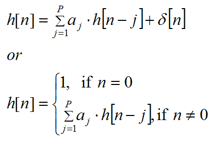
    1. When the LPC coefficients a_j are derived, you can construct impulse response signal
        h[n], 0≤n ≤ N-1 (N: frame size) by:

    2. The prediction Error E can be expressed by the autocorrelation function:

   3. The MatLab example code:

    x=[184.6400 184.1251 . . . . . . .  197.7890 -26.8000 ]; % original signal, dimension: frame size 

    y=[1.0000 2.0105  . . . . . . .   0.0738 0.0565 ]; % filter's impulse response h[n], dimension: frame size 

    gain=valG; %   valG: the prediction Error E

    X=fft(x,512); % fast Fourier Transform, so the frame size < 512

    Y=fft(y,512);  % fast Fourier Transform

    X(1)=[]; % remove the X(1), the DC

    Y(1)=[]; % remove the Y(1), the DC

   M=512;

   powerX=abs(X(1:M/2)).^2;  % the power spectrum of X

   logPX=10*log(powerX); % the power spectrum of X in dB

   powerY=abs(Y(1:M/2)).^2; % the power spectrum of Y

   logPY=10*log(powerY)+10*log(gain); % the power spectrum of Y in dB
                                                                   % plus   gain (Error) in dB
   nyquist=8000; % maximal frequency index

   freq=(1:M/2)/(M/2)*nyquist; % an array store the frequency indices

   figure(1);

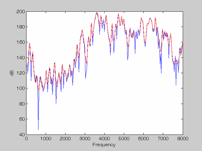
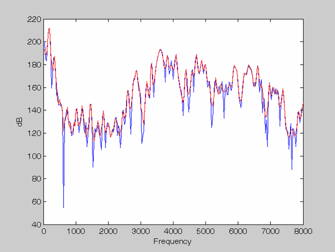
   plot(freq,logPX,'b',freq,logPY,'r'); % plot the result,
                                                           % b: blue line for the power spectrum of the original signal
                                                           % r: red line for the power spectrum of the filter

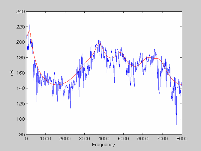
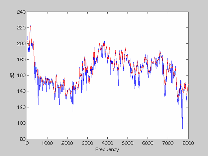
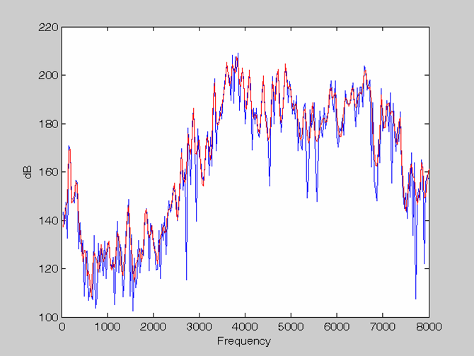
4. Example Figures of LPC Spectra (plotted by Roger Guo, Fall 2002)